Enhancing Ship Classification with CNNs and Switch Studying

Introduction

Welcome to an in-depth exploration of ship classification utilizing Convolutional Neural Networks (CNNs) with the Analytics Vidhya hackathon dataset. CNNs are a cornerstone of image-related duties, identified for his or her capability to study hierarchical representations of photos. On this challenge, we dive into understanding the ability of CNNs to categorise ships based mostly on their visible options.

This challenge goals to show deep studying software in picture categorization and examine CNNs constructed from scratch and people enhanced by way of switch studying. It explores ship classification, from preprocessing to analysis and comparability.

Studying Targets

• Apply Convolutional Neural Networks (CNNs) for ship classification.
• Preprocess picture knowledge utilizing OpenCV and NumPy.
• Implement CNN fashions each with and with out switch studying.
• Consider mannequin efficiency utilizing metrics like accuracy and F1-score.
• Evaluate the outcomes of CNN fashions with and with out switch studying.

Downside Assertion

On this context, the Governmental Maritime and Coastguard Company seeks to deploy an automatic ship detection system leveraging pc imaginative and prescient expertise. The target is to establish and classify ships from photos captured by survey boats precisely. With a various vary of ship sorts, together with cargo ships, tankers, army vessels, carriers, and cruise ships, the problem lies in growing a strong mannequin able to distinguishing between these lessons successfully.

Dataset Description

The 5 ship sorts—Cargo, Tanker, Army, Service, and Cruise—are represented within the dataset by a bunch of photographs taken by survey boats. The dataset gives all kinds of visible knowledge for mannequin development, with 6252 photos for coaching and 2680 photos for testing.

Rationalization of OpenCV and CNN

Allow us to discover about OpenCV and CNN intimately:

OpenCV

With its many options for picture processing duties together with object detection, function extraction, and film modifying, OpenCV is a potent software. We will enhance high quality of enter photographs, establish pertinent options, and preprocess the uncooked picture knowledge through the use of OpenCV.

Convolutional Neural Networks

CNNs are particularly designed for image-related duties. CNNs are significantly good at mechanically extracting options at numerous levels of abstraction from hierarchical representations of photos. We will create a mannequin that may acknowledge distinctive patterns and traits related to every sort of ship by coaching a CNN with the labeled ship photographs.

Layers in CNNs

CNNs include a number of layers, every serving a selected goal in processing and extracting options from enter photos. Let’s break down the elements of a CNN:

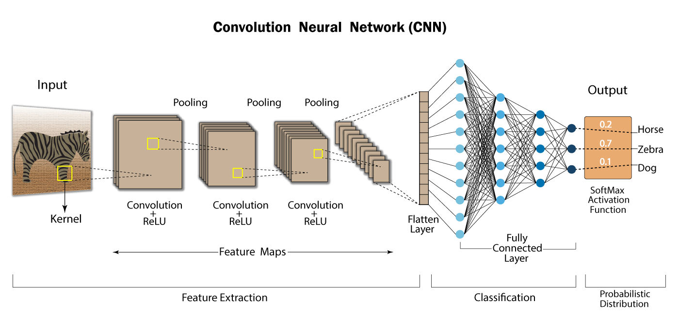
Convolutional Layers

CNNs are largely composed of convolutional layers. These layers are made up of learnable filters, generally known as kernels, which conduct convolution operations on the enter picture by sliding over it. The filters use element-wise multiplication and summing operations to extract completely different options from the enter picture, together with edges, textures, and patterns. Usually, every convolutional layer makes use of a variety of filters to gather numerous options.

Activation Perform

So as to add non-linearity to the community, an activation perform is utilized element-by-element to the output function maps following the convolution operation. Tanh, sigmoid, and ReLU (Rectified Linear Unit) are examples of frequent activation features. ReLU’s ease of use and effectivity in fixing the vanishing gradient concern make it essentially the most broadly utilized activation perform in CNNs.

Pooling Layers

Pooling layers downsample the function maps produced by the convolutional layers to protect essential info whereas lowering their spatial dimensions. The most well-liked pooling process, max pooling, successfully highlights salient options by retaining the utmost worth inside every pooling area. Pooling the enter reduces the community’s computational complexity and enhances its capability to study sturdy traits, making it extra resilient to slight spatial fluctuations.

Absolutely Related Layers

Absolutely related layers usually carry out classification or regression duties based mostly on the discovered options after the convolutional and pooling layers. These layers set up connections between every neuron in a layer and each different layer’s neuron, enabling the community to know the relationships between options extracted from the enter photos. Within the remaining phases of community development, totally related layers are sometimes used to generate the specified output, similar to class chances in picture classification duties.

Softmax Layer

Usually, a softmax layer is inserted on the finish of the community to remodel the category chances from the uncooked output scores in classification duties. To make sure that the output scores add as much as one and may be understood as chances, the softmax perform normalizes the values for every class. Consequently, the community can select the category with the very best likelihood to make predictions.

CNNs leverage convolutional layers with learnable filters to extract hierarchical options from enter photos, adopted by activation features to introduce non-linearity, pooling layers to downsample function maps, totally related layers for high-level function illustration, and a softmax layer for classification duties. This structure permits CNNs to carry out good in numerous image-related duties, together with picture classification, object detection, and segmentation.

Allow us to now apply the ideas to the dataset from the Analytics Vidhya hackathon.

Implementation of CNN

We’ll execute CNN implementation each with and with out switch studying. To start, let’s first sort out the implementation with out switch studying.

Right here’s the step-by-step implementation:

Step1: Importing Libraries and Dependencies

As we all know , the very first step is to put in all crucial libraries and dependencies:

import pandas as pd
import numpy as np
import cv2
import seaborn as sns
import tensorflow as tf
import matplotlib.pyplot as plt
from sklearn.model_selection import train_test_split
from tensorflow.keras.fashions import Sequential
from tensorflow.math import confusion_matrix
from tensorflow.keras.callbacks import ModelCheckpoint
from tensorflow.keras.layers import Conv2D, MaxPooling2D, Flatten, Dense, InputLayer
from glob import glob
from skimage.rework import resize
from keras.utils import to_categorical
from keras.fashions import Sequential
import keras
from keras.layers import Dense, Conv2D, MaxPool2D , Flatten
from tensorflow.keras import fashions, layers

Step2: Load the Dataset

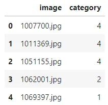
knowledge = pd.read_csv('/kaggle/enter/shipdataset/practice.csv')

Step3: Information Evaluation

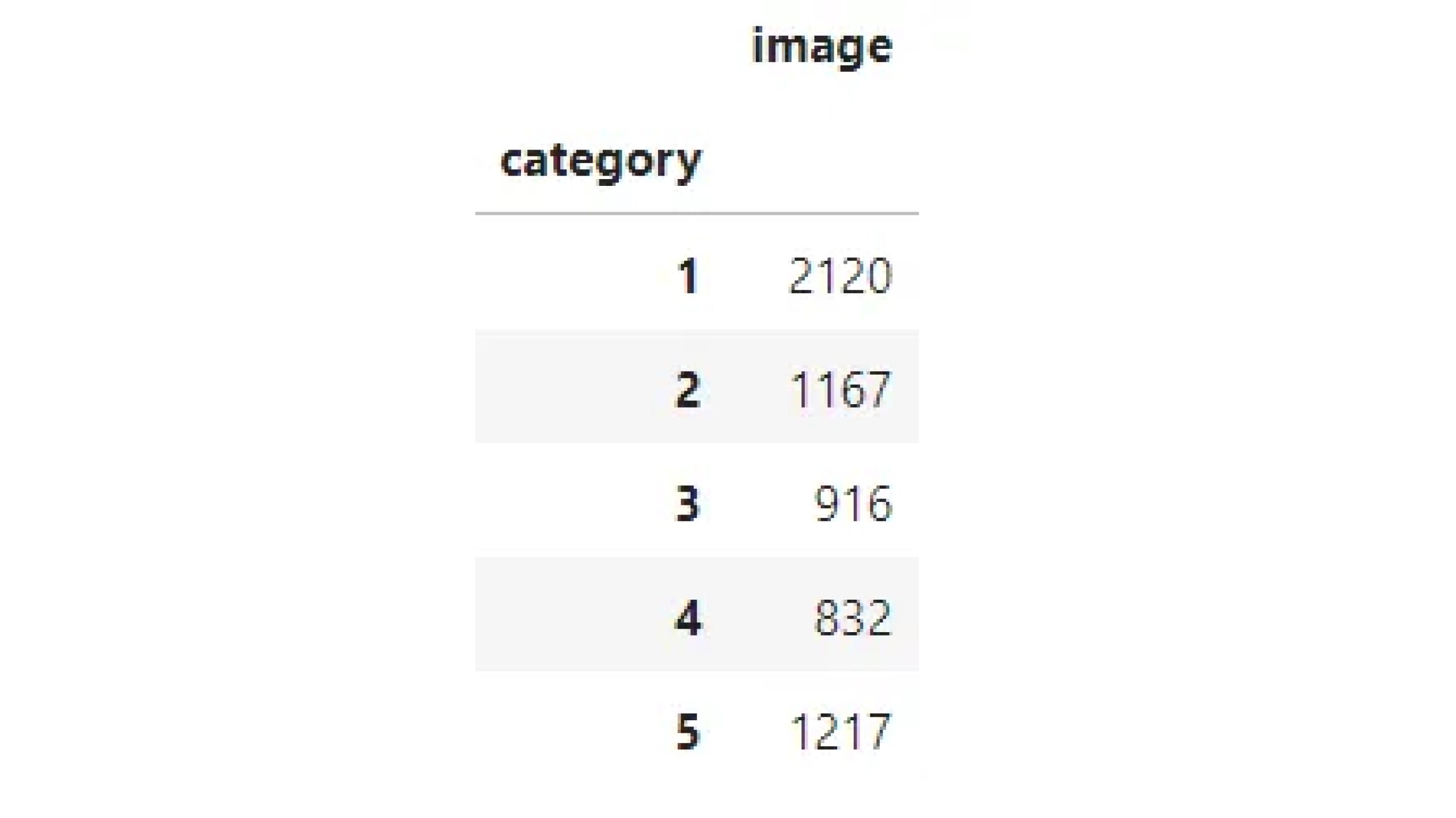
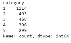
Now, let’s conduct some knowledge evaluation:

knowledge.groupby('class').depend()

This can present insights into the distribution of classes inside the dataset.

Step4: Visualization

Let’s now visualize this:

ship_categories = {1: 'Cargo', 2: 'Army', 3: 'Service', 4: 'Cruise', 5: 'Tanker'}
knowledge['category_mapped'] = knowledge['category'].map(ship_categories)
sns.countplot(x='category_mapped', knowledge=knowledge)

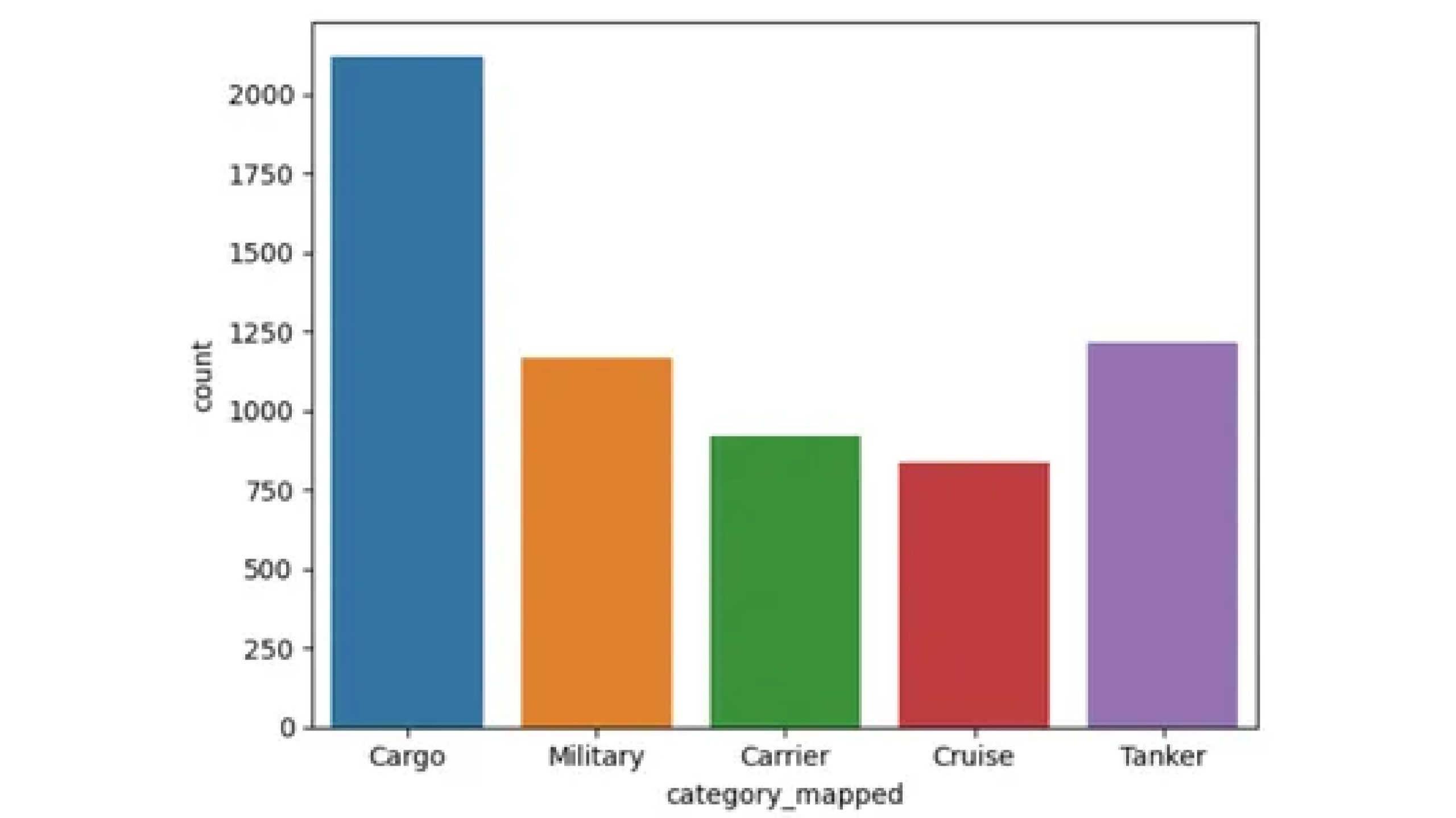
The countplot reveals that the dataset contains 2120 photos categorized as Cargo, 1167 as Army, 916 as Service, 832 as Cruise, and 1217 as Tanker.

Step5: Preprocessing the information

Now let’s preprocess the information with the assistance of code under:

X=[]
import cv2
for img_name in knowledge.picture:
    img=cv2.imread('/kaggle/enter/shipdataset/photos/'+img_name)
    img_resized = cv2.resize(img, (224, 224))
    X.append(img_resized)

X=np.array(X)

This code hundreds photos from a listing, resizes them to 224×224 pixels utilizing OpenCV, and shops the resized photos in a NumPy array.

Step6: Plotting

Now let’s plot them after resizing.

nrow = 5
ncol = 4
fig1 = plt.determine(figsize=(15, 15))
fig1.suptitle('After Resizing', measurement=32)
for i in vary(20):
    plt.subplot(nrow, ncol, i + 1)
    plt.imshow(X[i])
    plt.title('class = {x}, Ship = {y}'.format(x=knowledge["category"][i],
     y=ship_categories[data["category"][i]]))
    plt.axis('Off')
    plt.grid(False)
plt.present()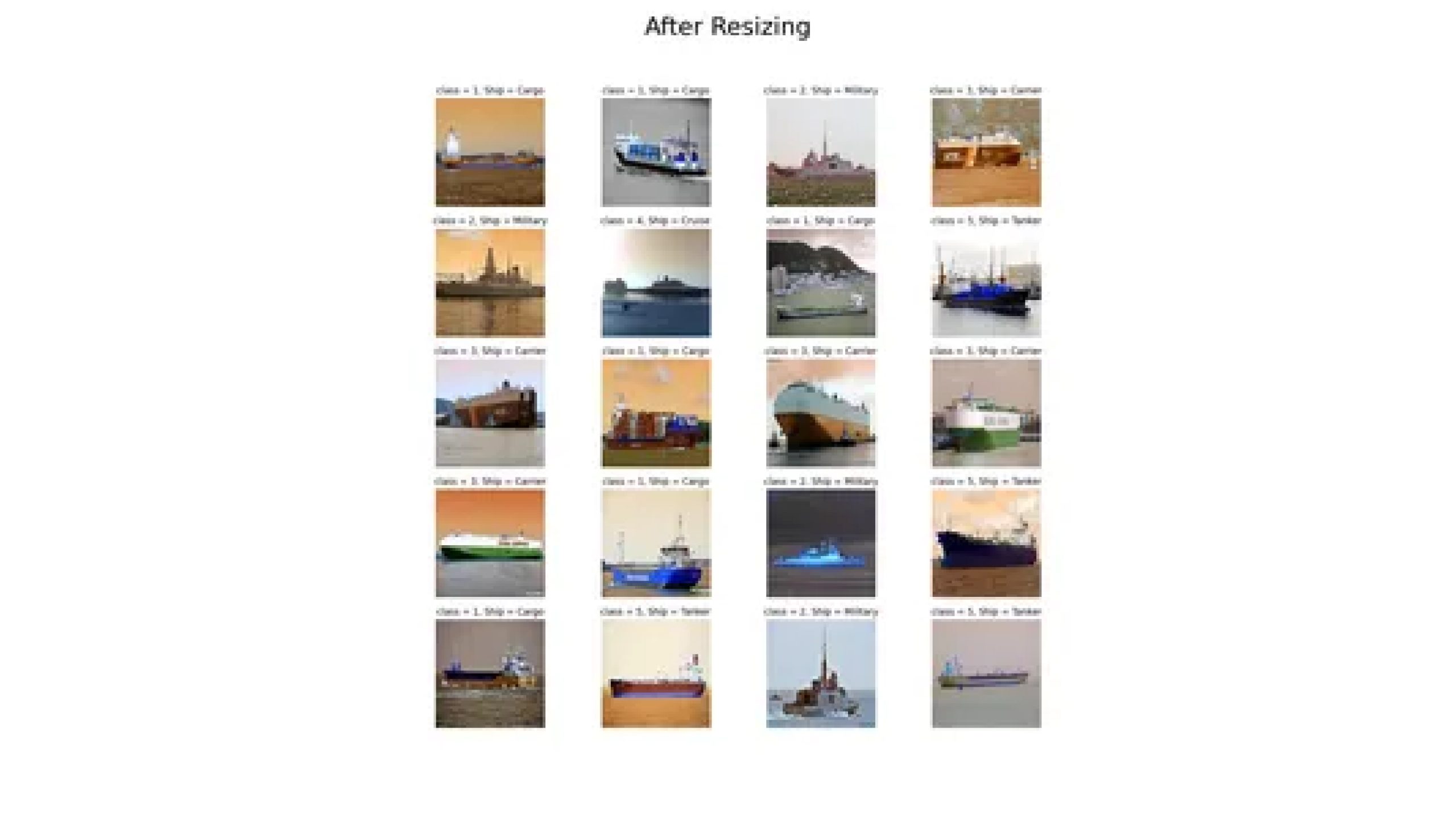

y=knowledge.class.values
y=y-1

This step subtracts 1 from every worth within the knowledge.class array, storing the outcome within the variable y.

The aim of this operation may very well be to regulate the class labels. It’s frequent in machine studying duties to begin indexing from 0 as a substitute of 1, particularly when coping with classification duties. To align the labels with zero-based indexing, subtracting 1 from the class labels is usually accomplished, as required by machine studying algorithms or libraries.

X = X.astype('float32') / 255
y = to_categorical(y)

This code converts pixel values in X to floats between 0 and 1 and one-hot encodes categorical labels in y.

Step7: Information Splitting into Prepare/Take a look at Dataset

Cut up the dataset into coaching and testing units utilizing the train_test_split perform.

X_train, X_test, y_train, y_test = train_test_split(X, y,
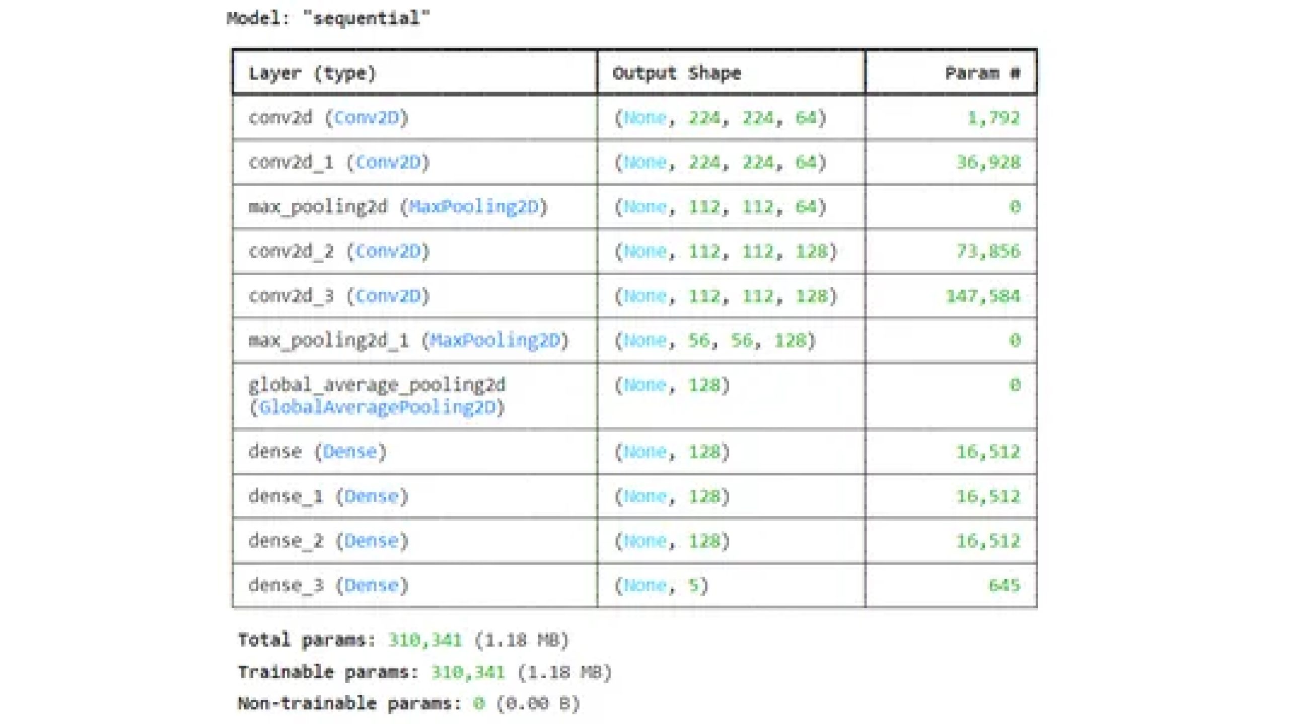
 test_size=0.2, random_state=42)

Defining CNN Mannequin: Outline a CNN mannequin utilizing TensorFlow’s Sequential API, specifying the convolutional and pooling layers.

CNN_model = fashions.Sequential([
    layers.Conv2D(64, (3, 3), activation='relu', padding='same', 
    input_shape=(224, 224, 3)),
    layers.Conv2D(64, (3, 3), padding='same', activation='relu'),
    layers.MaxPooling2D((2, 2)),
    layers.Conv2D(128, (3, 3), padding='same', activation='relu'),
    layers.Conv2D(128, (3, 3), padding='same', activation='relu'), 
    layers.MaxPooling2D((2, 2)),
    layers.GlobalAveragePooling2D(),  
    layers.Dense(128, activation='relu'),
    layers.Dense(128, activation='relu'),
    layers.Dense(128, activation='relu'),
    layers.Dense(5, activation='softmax')  
])
CNN_model.abstract()

Step8: Mannequin Coaching

rain the CNN mannequin on the coaching knowledge, organising early stopping and mannequin checkpoint to stop overfitting and save one of the best mannequin.

Compile the mannequin with adam optimizer and loss as categorical cross entropy because it’s multiclass classification

from tensorflow.keras.optimizers import Adam
mannequin.compile(optimizer="adam",
                  loss="categorical_crossentropy",
                  metrics=['accuracy',tf.keras.metrics.F1Score()])

Saving one of the best mannequin on validation loss

from tensorflow.keras.callbacks import EarlyStopping, ModelCheckpoint
early_stop = EarlyStopping(monitor="val_loss", 
persistence=3, restore_best_weights=True)
checkpoint = ModelCheckpoint('best_model.keras', 
monitor="val_loss", save_best_only=True, mode="min")

Step9: Becoming the Mannequin

historical past = mannequin.match(X_train, y_train, 
                        epochs=20, 
                        batch_size=32, 
                        validation_data=(X_test, y_test), 
                        callbacks=[early_stop, checkpoint])

Step10: Mannequin Analysis

Now let’s do mannequin analysis utilizing skilled mannequin.

from sklearn.metrics import f1_score
y_pred = mannequin.predict(X_test)

Changing predictions from one-hot encoded format to class labels.

y_pred_labels = np.argmax(y_pred, axis=1)
y_true_labels = np.argmax(y_test, axis=1)

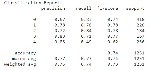
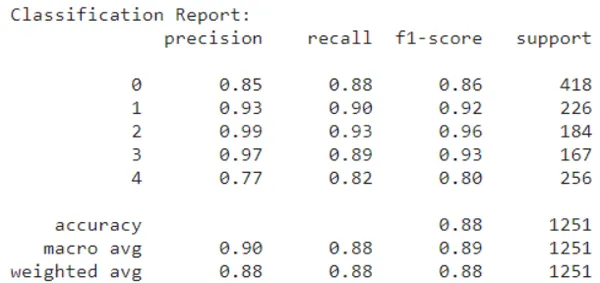
from sklearn.metrics import classification_report
report = classification_report(y_true_labels, y_pred_labels)
print("Classification Report:")
print(report)

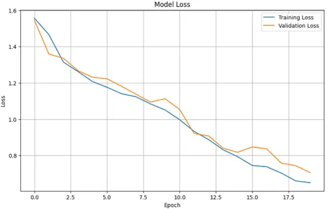
Plotting coaching & validation loss values

plt.determine(figsize=(10, 6))
plt.plot(historical past.historical past['loss'], label="Coaching Loss")
plt.plot(historical past.historical past['val_loss'], label="Validation Loss")
plt.title('Mannequin Loss')
plt.xlabel('Epoch')
plt.ylabel('Loss')
plt.legend()
plt.grid(True)
plt.present()

import matplotlib.pyplot as plt
plt.plot(historical past.historical past['accuracy'], label="Coaching accuracy")
plt.plot(historical past.historical past['val_accuracy'], label="Validation accuracy")
plt.title('Coaching and Validation accuracy')
plt.xlabel('Epoch')
plt.ylabel('Accuracy')
plt.legend()
plt.grid(True)
plt.present()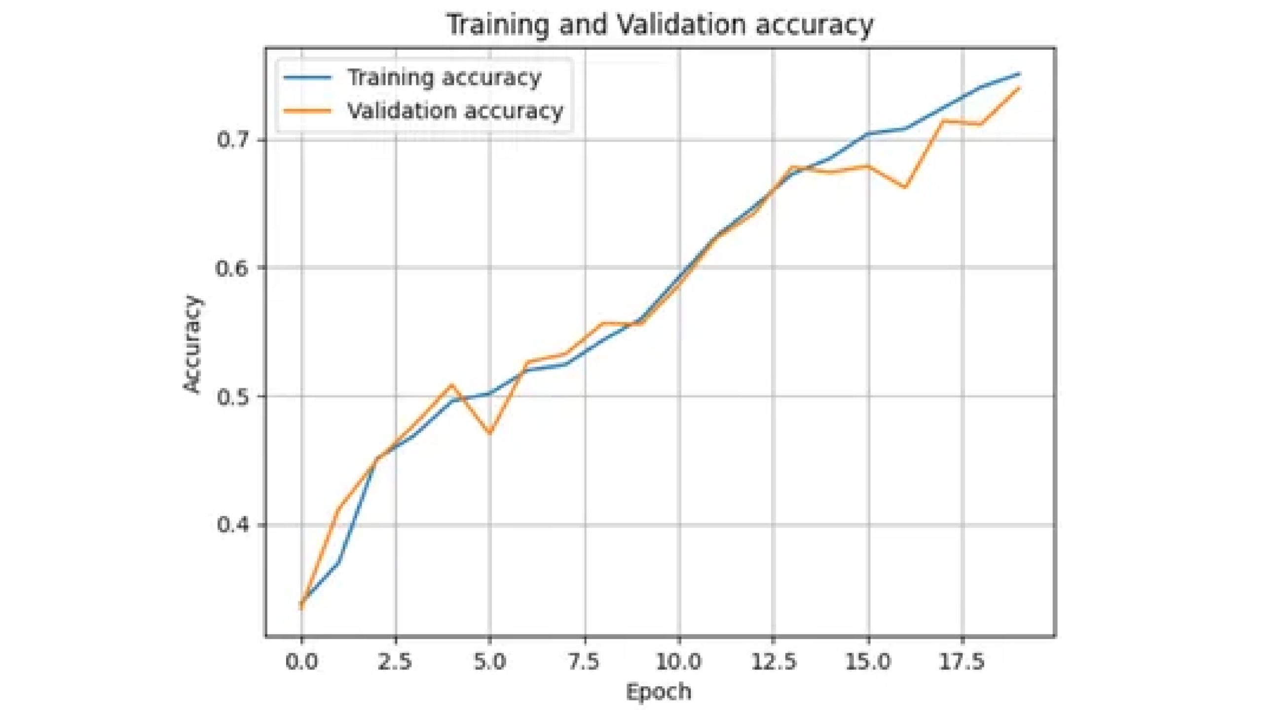

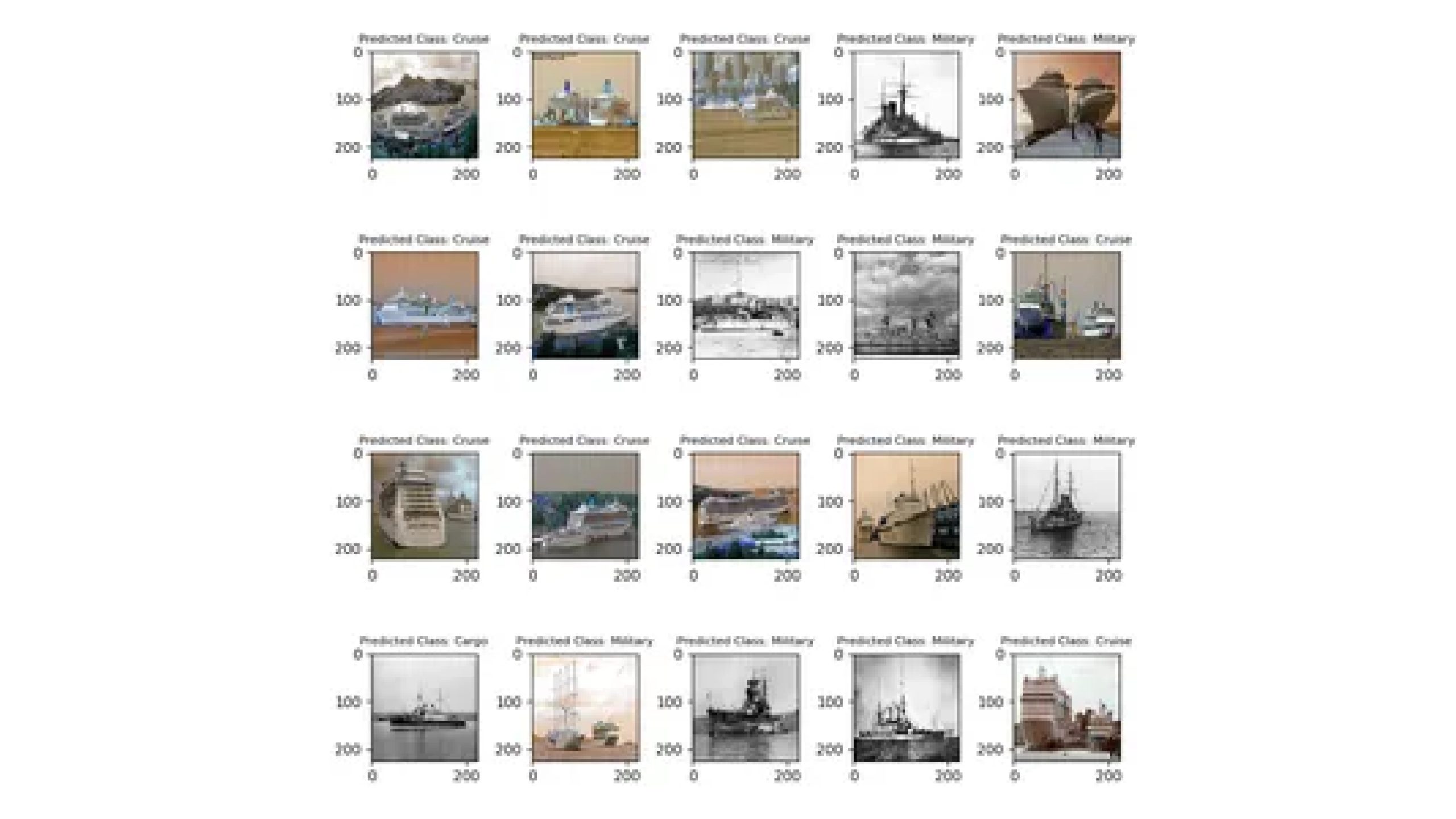
Testing of Information

Making ready and preprocessing the check knowledge equally to the coaching knowledge, make predictions utilizing the skilled mannequin, and visualize some pattern predictions together with their predicted lessons.

check=pd.read_csv('/kaggle/enter/test-data/test_ApKoW4T.csv')

X_test=[]
import cv2
for img_name in check.picture:
    img=cv2.imread('/kaggle/enter/shipdataset/photos/'+img_name)
    img_resized = cv2.resize(img, (224, 224))
    X_test.append(img_resized)
X_test=np.array(X_test)
X_test = X_test.astype('float32') / 255

Making Prediction

predictions=mannequin.predict(X_test)
predicted_class= np.argmax(predictions,axis=1)
predicted_class=predicted_class+1
csv_=check.copy()
csv_
csv_['category']=predicted_class
csv_.head()

csv_['category'].value_counts()

Save Predictions in CSV

csv_.to_csv('prediction1.csv',index=False)

Plotting the Predicted Take a look at Information

plt.determine(figsize=(8, 8))
for i in vary(20):
    plt.subplot(4, 5, i + 1)  
    plt.imshow(X_test[i])  
    plt.title(f'Predicted Class: {ship_categories[predicted_class[i]]}', fontsize=8)  
plt.tight_layout() 
plt.savefig('prediction_plot1.png')
plt.present()

Now let’s use switch studying to resolve this downside for this we might be utilizing resnet.

Understanding Mobilenet

Mobilenet is a kind of convolutional neural community (CNN) designed particularly for cellular and embedded gadgets . It’s identified for being environment friendly and light-weight, making it excellent for conditions the place processing energy and battery life are restricted.

Right here’s a breakdown of Mobilenet’s key options:

• Effectivity: Mobilenet employs depthwise separable convolutions, which divide knowledge processing into two steps: depthwise convolution utilizing a single filter for every enter channel and pointwise convolution utilizing 1×1 filters.
• Light-weight: Mobilenet lowers the quantity of parameters wanted by the mannequin by minimizing computations. Which means the mannequin might be smaller, which is essential for cellular gadgets with constrained storage.
• Functions: It’s helpful for numerous duties on cellular gadgets, together with picture classification, object detection, and facial recognition.

You possibly can learn extra about MobileNet by clicking right here.

We are going to make the most of MobileNet for this activity. The whole lot stays constant from importing libraries to knowledge splitting(identical step as with out switch studying) . Moreover, we have to import the MobileNet library.

from keras.purposes import MobileNet
from keras.fashions import Mannequin
from keras.layers import Dense, GlobalAveragePooling2D
from keras.layers import Dropout, BatchNormalization

Loading Pre-trained Mannequin

Now load the Pre-trained Mannequin as base mannequin

base_model = MobileNet(weights="imagenet", include_top=False)

Freeze all layers within the base mannequin:

for layer in base_model.layers:
    layer.trainable = False

Construct Mannequin Utilizing Purposeful Perform 

x = base_model.output
x = GlobalAveragePooling2D()(x)
x = Dense(1024, activation='relu')(x)
x = BatchNormalization()(x)
x = Dropout(0.5)(x)  # Add dropout with a charge of 0.5
predictions = Dense(5, activation='softmax')(x)
 
#Creating the mannequin
mannequin = Mannequin(inputs=base_model.enter, outputs=predictions)

Compiling the Mannequin

Compile the mannequin with adam optimizer and loss as categorical cross entropy because it’s multiclass classification

from tensorflow.keras.optimizers import Adam
mannequin.compile(optimizer="adam",
                  loss="categorical_crossentropy",
                  metrics=['accuracy',tf.keras.metrics.F1Score()])

Saving the Finest Mannequin on Validation Loss

from tensorflow.keras.callbacks import EarlyStopping, ModelCheckpoint
early_stop = EarlyStopping(monitor="val_loss", persistence=2, restore_best_weights=True)
checkpoint = ModelCheckpoint('best_model.keras', monitor="val_loss", 
  save_best_only=True, mode="min")

Becoming the Mannequin

historical past = mannequin.match(X_train, y_train, 
                    epochs=20, 
                    batch_size=32, 
                    validation_data=(X_test, y_test),
                    callbacks=[early_stop,checkpoint])

Mannequin Analysis

Now let’s do mannequin analysis.

from sklearn.metrics import f1_score

#Making predictions utilizing the skilled mannequin
y_pred = mannequin.predict(X_test)

#Changing predictions from one-hot encoded format to class labels
y_pred_labels = np.argmax(y_pred, axis=1)
y_true_labels = np.argmax(y_test, axis=1)

from sklearn.metrics import classification_report
report = classification_report(y_true_labels, y_pred_labels)
print("Classification Report:")
print(report)

Plotting Coaching and Validation Loss Values

plt.determine(figsize=(10, 6))
plt.plot(historical past.historical past['loss'], label="Coaching Loss")
plt.plot(historical past.historical past['val_loss'], label="Validation Loss")
plt.title('Mannequin Loss')
plt.xlabel('Epoch')
plt.ylabel('Loss')
plt.legend()
plt.grid(True)
plt.present()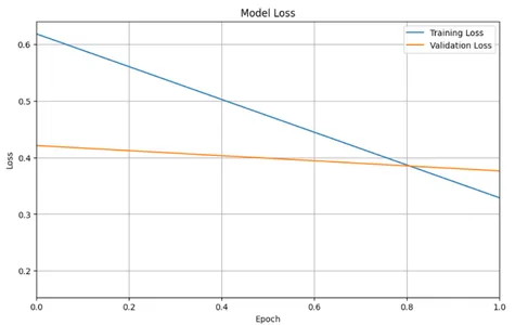

Plotting Accuracy Curve

import matplotlib.pyplot as plt
plt.plot(historical past.historical past['accuracy'], label="Coaching accuracy")
plt.plot(historical past.historical past['val_accuracy'], label="Validation accuracy")
plt.title('Coaching and Validation accuracy')
plt.xlabel('Epoch')
plt.ylabel('Accuracy')
plt.legend()
plt.grid(True)
plt.present()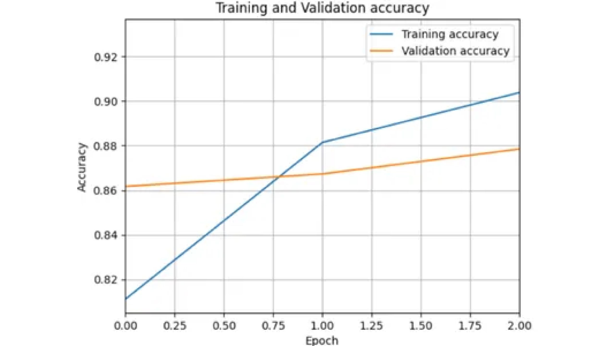

Now do the prediction on check knowledge identical as accomplished in with out switch studying

Conclusion

This research explores two approaches to ship classification utilizing Convolutional Neural Networks (CNNs). The primary includes constructing a CNN from scratch with out switch studying strategies, whereas the second makes use of switch studying utilizing MobileNet structure. Each strategies present potential options for ship classification, with switch studying providing higher efficiency with much less coaching knowledge. The selection is determined by computational sources, dataset measurement, and desired efficiency metrics.

Steadily Requested Questions