How Knowledge Environment friendly GANs Generate Photos of Cats and Canine?

Introduction

Generative adversarial networks are a well-liked framework for Picture era. On this article we’ll practice Knowledge-efficient GANs with Adaptive Discriminator Augmentation that addresses the problem of restricted coaching knowledge. Adaptive Discriminator Augmentation dynamically adjusts knowledge augmentation throughout GAN coaching, stopping discriminator overfitting and enhancing mannequin generalization. By using invertible augmentation strategies and probabilistic software, ADA ensures compatibility with GAN dynamics whereas sustaining the info distribution. This text will discover Adaptive Discriminator Augmentations transformative impression on GAN effectivity and picture era high quality.

Studying Aims

• Perceive the basics of Generative Adversarial Networks and their function in picture era.
• Discover ways to load and preprocess knowledge utilizing TensorFlow for GAN coaching.
• Acknowledge the challenges posed by restricted coaching knowledge in GANs and the significance of addressing discriminator overfitting.
• Implement Adaptive Discriminator Augmentation (ADA) method to reinforce GAN coaching effectivity and enhance picture era high quality.
• Acquire proficiency in producing photos utilizing GANs and consider their high quality utilizing metrics like Kernel Inception Distance (KID).
• Purchase sensible abilities in setting hyperparameters, loading datasets, and implementing pre-trained fashions like InceptionV3 inside GAN coaching pipelines.

What are GANs?

Generative Adversarial Networks (GANs) characterize a major development within the realm of unsupervised studying throughout the area of synthetic intelligence. Comprising two distinct neural networks – a discriminator and a generator – GANs function on the precept of adversarial coaching to generate artificial knowledge carefully resembling real-world samples. The crux of their operation lies within the aggressive interaction between these networks, the place the generator endeavors to deceive the discriminator by producing more and more practical outputs from random noise inputs.

GANs are a kind of knowledge era system that makes use of probabilistic fashions to seize patterns and buildings in datasets. The adversarial part of GANs includes pitting generator outputs in opposition to genuine knowledge, with a discriminator discerning between the 2. The generator refines its output to approximate real-world knowledge, whereas the discriminator evolves to differentiate extra precisely. GANs use deep neural networks to coach and optimize their architectures, showcasing their computational prowess and using AI algorithms.

Structure of GANs

On this article we gained’t take a look at the in-depth working of a GAN, we’ll deal with the implementation a part of it. Right here’s a excessive degree overview of GANs:

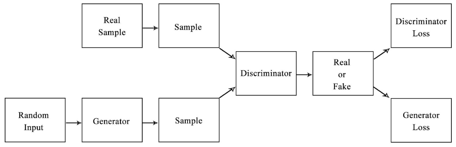
Generative Adversarial Networks include two important elements: the Generator and the Discriminator.

• Generator Mannequin: The generator creates practical knowledge from random noise, adjusting its parameters by means of coaching to imitate actual samples. It’s purpose is to idiot the Discriminator.
• Discriminator Mannequin: Differentiates between actual and generated knowledge, enhancing over time to precisely establish pretend samples. Its interplay with the Generator enhances GAN’s potential to supply practical knowledge.

What’s Knowledge Environment friendly GANs?

Knowledge Environment friendly GANs with Adaptive Discriminator Augmentation improves GAN coaching addresses discriminator overfitting resulting from restricted knowledge. Conventional GANs wrestle with restricted knowledge, because the generator may not obtain helpful suggestions from the discriminator. Right here we’ll use adaptive knowledge augmentation for the discriminator, making certain it doesn’t overfit. This augmentation is utilized in a differentiable and GPU-compatible method, essential for GAN coaching. Moreover, invertible knowledge augmentation prevents “leaky augmentations” by making use of transformations with some likelihood, preserving the unique knowledge distribution and enhancing discriminator regularization.

Producing Photos Utilizing GAN

On this article we’ll be working with “cats_vs_dogs” dataset from tensorflow, in the event you select to work with different datasets from tensorflow you’ll be able to take a look at the accessible datasets utilizing “tfds.list_builders()”.

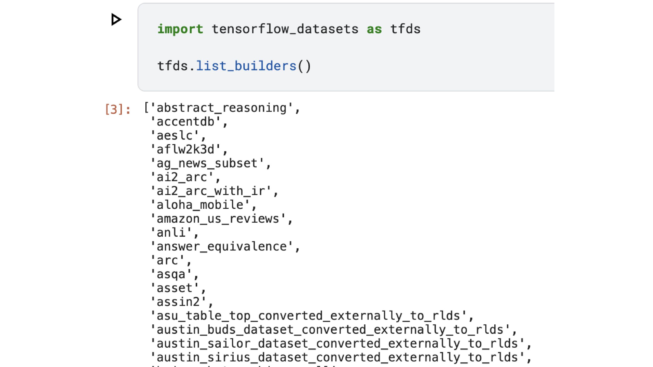
You possibly can see extra about Cats_vs_Dogs dataset right here.

Step1: Import the Obligatory Modules

Let’s begin by loading the info, however earlier than that permit’s do some needed imports. 

import matplotlib.pyplot as plt
import tensorflow as tf
import tensorflow_datasets as tfds
from tensorflow import keras
from keras import layers

Be aware: It’s endorsed to replace your tensorflow and tensorflow-datasets earlier than we begin:

Step2: Loading the Dataset

!pip set up --upgrade tensorflow
!pip set up --upgrade tensorflow-datasets
Setting Hyperparameters
num_epochs = 500
image_size = 64
dataset_name = "cats_vs_dogs" 
kid_image_size = 75
padding = 0.25
# adaptive discriminator augmentation
max_translation = 0.125
max_rotation = 0.125
max_zoom = 0.25
target_accuracy = 0.85
integration_steps = 1000
# structure
noise_size = 64
depth = 4
width = 128
leaky_relu_slope = 0.2
dropout_rate = 0.4
# optimization
batch_size = 128
learning_rate = 2e-4
beta_1 = 0.5  
ema = 0.99
Loading the info 
def round_to_int(float_value):
    return tf.forged(tf.math.spherical(float_value), dtype=tf.int32)

def preprocess_image(knowledge):
    # Resize and normalize photos
    picture = tf.picture.resize(knowledge['image'], [image_size, image_size])
    picture = tf.forged(picture, tf.float32) / 255.0
    return picture
def prepare_dataset(cut up):
    # Load dataset, preprocess photos, and apply shuffling and batching
    return (
        tfds.load(dataset_name, cut up="practice", shuffle_files=True)
        .map(preprocess_image, num_parallel_calls=tf.knowledge.AUTOTUNE)
        .cache()
        .shuffle(10 * batch_size)
        .batch(batch_size, drop_remainder=True)
        .prefetch(buffer_size=tf.knowledge.AUTOTUNE)
    )
train_dataset = prepare_dataset("practice")
val_dataset = train_dataset
Let’s take a look at the photographs:
import matplotlib.pyplot as plt
def show_images(dataset, num_images=5):
    plt.determine(figsize=(10, 10))
    for photos in dataset.take(1):
        for i in vary(num_images):
            ax = plt.subplot(1, num_images, i + 1)
            plt.imshow(photos[i])
            plt.axis("off")
# Show photos from practice and validation dataset
show_images(train_dataset)
show_images(val_dataset)
plt.present()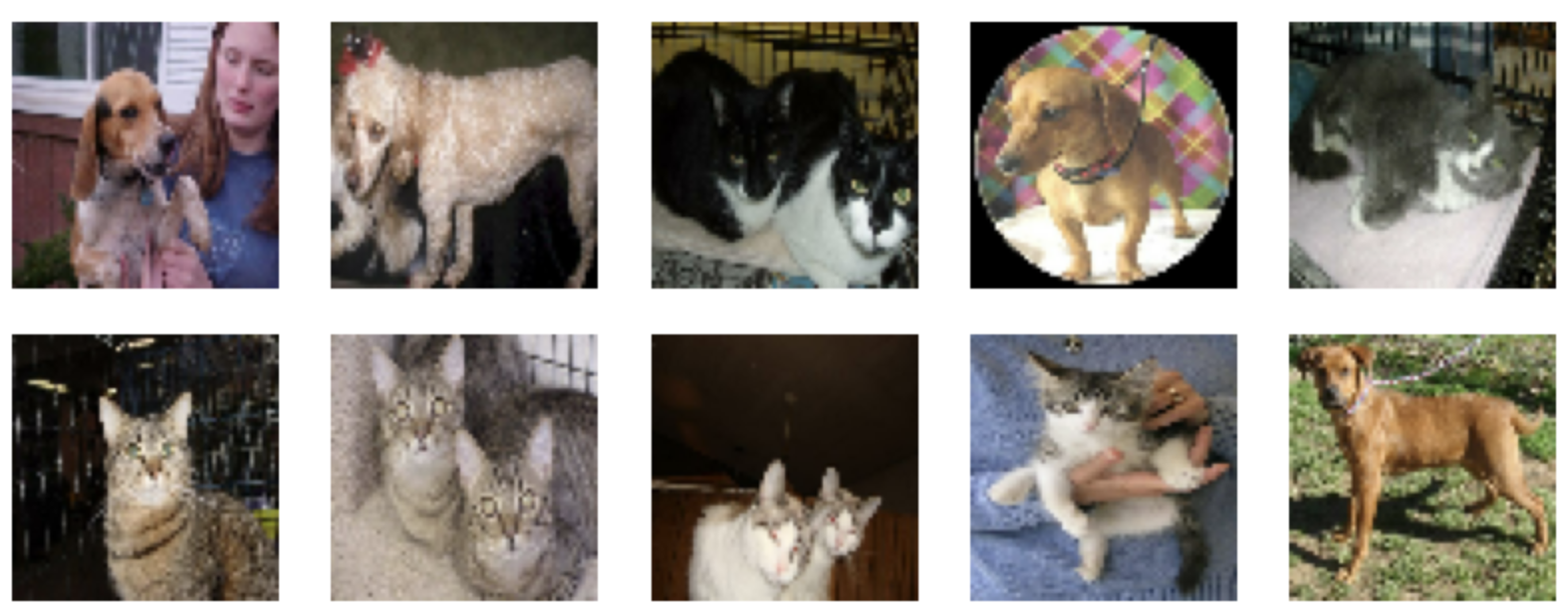

Step3: Utilizing Pre-trained Mannequin

We’ll be utilizing a pre-trained InceptionV3 mannequin together with the GAN, however we gained’t be utilizing the classification layer of the InceptionV3.

Kernel Inception Distance (KID) measures picture era high quality primarily based on variations in InceptionV3 community representations. It’s computationally environment friendly and unbiased, appropriate for small datasets, estimating per-batch and averaging throughout batches.

class KID(keras.metrics.Metric):
   def __init__(self, identify="child", **kwargs):
       tremendous().__init__(identify=identify, **kwargs)
       # KID is estimated per batch and is averaged throughout batches
       self.kid_tracker = keras.metrics.Imply()
       # Utilizing a pretrained InceptionV3 is used with out the classification layer
       self.encoder = keras.Sequential(
           [
               layers.InputLayer(input_shape=(image_size, image_size, 3)),
               layers.Rescaling(255.0),
               layers.Resizing(height=kid_image_size, width=kid_image_size),
               layers.Lambda(keras.applications.inception_v3.preprocess_input),
               keras.applications.InceptionV3(
                   include_top=False,
                   input_shape=(kid_image_size, kid_image_size, 3),
                   weights="imagenet",
               ),
               layers.GlobalAveragePooling2D(),
           ],
           identify="inception_encoder",
       )
   def polynomial_kernel(self, features_1, features_2):
       feature_dimensions = tf.forged(tf.form(features_1)[1], dtype=tf.float32)
      return (features_1 @ tf.transpose(features_2) / feature_dimensions + 1.0) ** 3.0
   def update_state(self, real_images, generated_images, sample_weight=None):
       real_features = self.encoder(real_images, coaching=False)
       generated_features = self.encoder(generated_images, coaching=False)
       # compute polynomial kernels utilizing the 2 units of options
       kernel_real = self.polynomial_kernel(real_features, real_features)
       kernel_generated = self.polynomial_kernel(
           generated_features, generated_features

       )

       kernel_cross = self.polynomial_kernel(real_features, generated_features)
       # estimate the squared most imply discrepancy utilizing the typical kernel values
       batch_size = tf.form(real_features)[0]

       batch_size_f = tf.forged(batch_size, dtype=tf.float32)
      mean_kernel_real = tf.reduce_sum(kernel_real * (1.0 - tf.eye(batch_size))) / (
           batch_size_f * (batch_size_f - 1.0)
       )
       mean_kernel_generated = tf.reduce_sum(
           kernel_generated * (1.0 - tf.eye(batch_size))
       ) / (batch_size_f * (batch_size_f - 1.0))
       mean_kernel_cross = tf.reduce_mean(kernel_cross)
       child = mean_kernel_real + mean_kernel_generated - 2.0 * mean_kernel_cross
       # replace the typical KID estimate
       self.kid_tracker.update_state(child)

   def end result(self):
       return self.kid_tracker.end result()

   def reset_state(self):
       self.kid_tracker.reset_state()

Step4: Augmenter, Discriminator and Generator

Adaptive discriminator augmentation used right here adjusts augmentation likelihood throughout coaching by way of integral management to take care of discriminator accuracy on actual photos close to a goal worth.

# "arduous sigmoid", helpful for binary accuracy calculation from logits
def step(values):
   # damaging values -> 0.0, constructive values -> 1.0
   return 0.5 * (1.0 + tf.signal(values))
# augments photos with a likelihood that's dynamically up to date throughout coaching
class AdaptiveAugmenter(keras.Mannequin):
   def __init__(self):
       tremendous().__init__()
       # shops the present likelihood of a picture being augmented
       self.likelihood = tf.Variable(0.0)
       # the corresponding augmentation names from the paper are proven above every layer
       # the authors present (see determine 4), that the blitting and geometric augmentations
       # are essentially the most useful within the low-data regime
       self.augmenter = keras.Sequential(
           [
               layers.InputLayer(input_shape=(image_size, image_size, 3)),
               # blitting/x-flip:
               layers.RandomFlip("horizontal"),
               # blitting/integer translation:
               layers.RandomTranslation(
                   height_factor=max_translation,
                   width_factor=max_translation,
                   interpolation="nearest",
               ),
               # geometric/rotation:
               layers.RandomRotation(factor=max_rotation),
               # geometric/isotropic and anisotropic scaling:
               layers.RandomZoom(
                   height_factor=(-max_zoom, 0.0), width_factor=(-max_zoom, 0.0)
               ),
           ],
           identify="adaptive_augmenter",
       )
   def name(self, photos, coaching):
       if coaching:
           augmented_images = self.augmenter(photos, coaching)
           # throughout coaching both the unique or the augmented photos are chosen
           # primarily based on self.likelihood
           augmentation_values = tf.random.uniform(
               form=(batch_size, 1, 1, 1), minval=0.0, maxval=1.0
           )
           augmentation_bools = tf.math.much less(augmentation_values, self.likelihood)
           photos = tf.the place(augmentation_bools, augmented_images, photos)
       return photos
   def replace(self, real_logits):
       current_accuracy = tf.reduce_mean(step(real_logits))
       # the augmentation likelihood is up to date primarily based on the discriminator's
       # accuracy on actual photos
       accuracy_error = current_accuracy - target_accuracy
       self.likelihood.assign(
           tf.clip_by_value(
               self.likelihood + accuracy_error / integration_steps, 0.0, 1.0
           )
       )
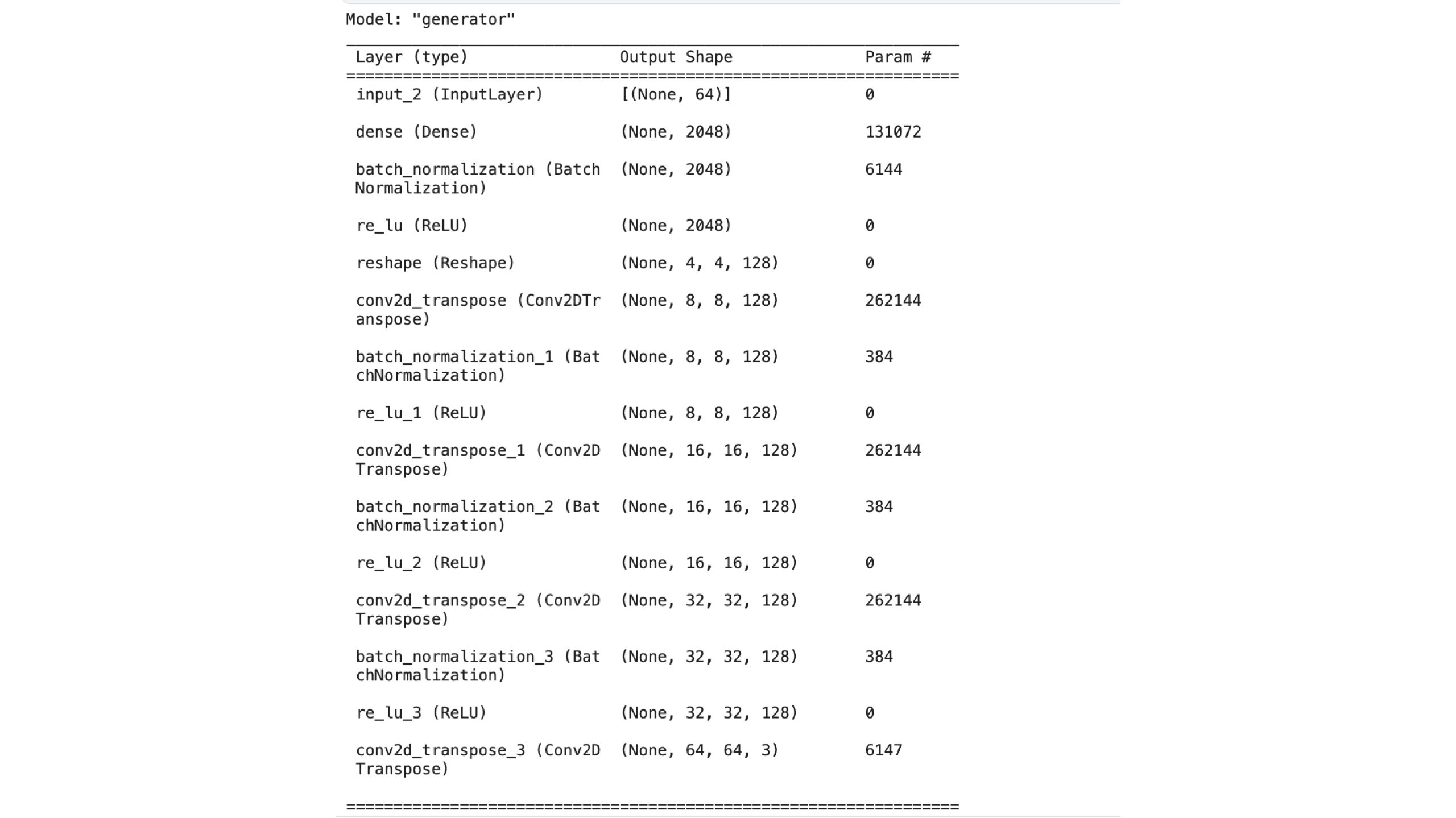
We’ll be utilizing the tried and examined Deeply related GAN’s (DC-GAN) generator and discriminator. 

def get_generator():
   noise_input = keras.Enter(form=(noise_size,))
   x = layers.Dense(4 * 4 * width, use_bias=False)(noise_input)
   x = layers.BatchNormalization(scale=False)(x)
   x = layers.ReLU()(x)
   x = layers.Reshape(target_shape=(4, 4, width))(x)
   for _ in vary(depth - 1):
       x = layers.Conv2DTranspose(
           width, kernel_size=4, strides=2, padding="identical", use_bias=False,
       )(x)
       x = layers.BatchNormalization(scale=False)(x)
       x = layers.ReLU()(x)
   image_output = layers.Conv2DTranspose(
       3, kernel_size=4, strides=2, padding="identical", activation="sigmoid",
   )(x)
   return keras.Mannequin(noise_input, image_output, identify="generator")
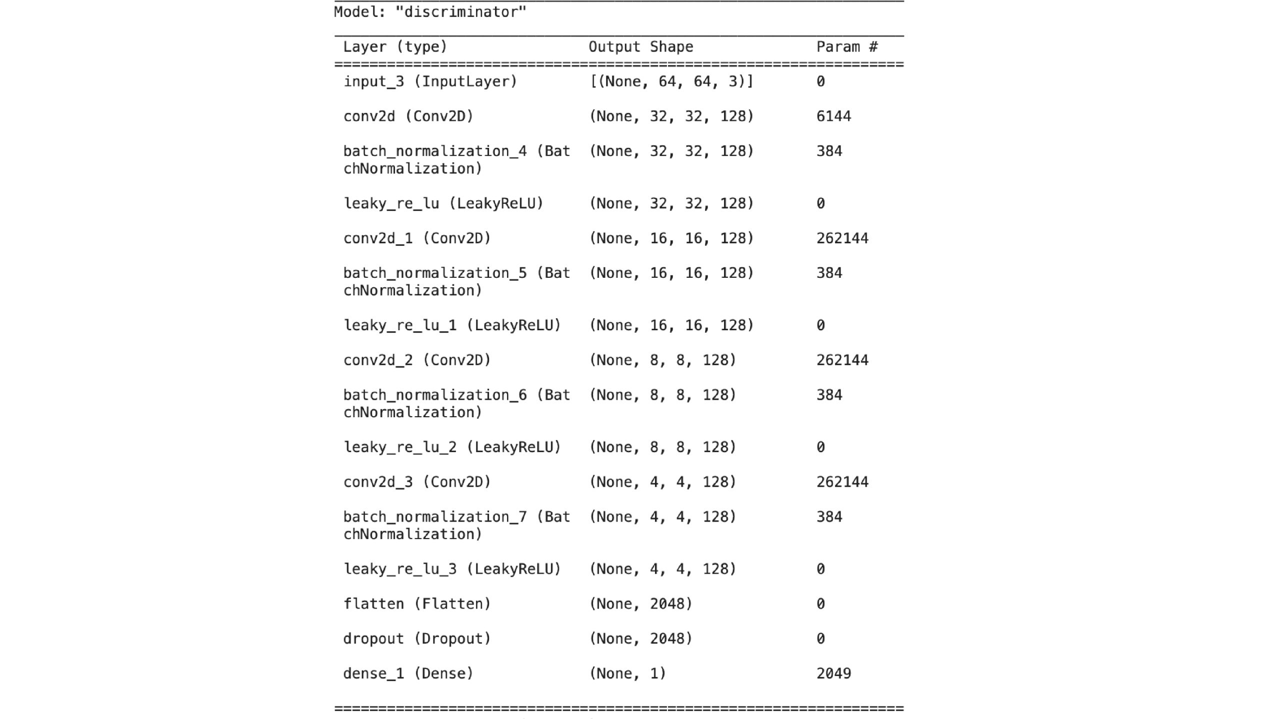
# DCGAN discriminator
def get_discriminator():
   image_input = keras.Enter(form=(image_size, image_size, 3))
   x = image_input
   for _ in vary(depth):
       x = layers.Conv2D(
           width, kernel_size=4, strides=2, padding="identical", use_bias=False,
       )(x)
       x = layers.BatchNormalization(scale=False)(x)
       x = layers.LeakyReLU(alpha=leaky_relu_slope)(x)
   x = layers.Flatten()(x)
   x = layers.Dropout(dropout_rate)(x)
   output_score = layers.Dense(1)(x)
   return keras.Mannequin(image_input, output_score, identify="discriminator")
class GAN_ADA(keras.Mannequin):
   def __init__(self):
       tremendous().__init__()
       self.augmenter = AdaptiveAugmenter()
       self.generator = get_generator()
       self.ema_generator = keras.fashions.clone_model(self.generator)
       self.discriminator = get_discriminator()
       self.generator.abstract()
       self.discriminator.abstract()
   def compile(self, generator_optimizer, discriminator_optimizer, **kwargs):
       tremendous().compile(**kwargs)
       # separate optimizers for the 2 networks
       self.generator_optimizer = generator_optimizer
       self.discriminator_optimizer = discriminator_optimizer
       self.generator_loss_tracker = keras.metrics.Imply(identify="g_loss")
       self.discriminator_loss_tracker = keras.metrics.Imply(identify="d_loss")
       self.real_accuracy = keras.metrics.BinaryAccuracy(identify="real_acc")
       self.generated_accuracy = keras.metrics.BinaryAccuracy(identify="gen_acc")
       self.augmentation_probability_tracker = keras.metrics.Imply(identify="aug_p")
       self.child = KID()
   @property
   def metrics(self):
       return [
           self.generator_loss_tracker,
           self.discriminator_loss_tracker,
           self.real_accuracy,
           self.generated_accuracy,
          self.augmentation_probability_tracker,
           self.kid,
       ]
   def generate(self, batch_size, coaching):
       latent_samples = tf.random.regular(form=(batch_size, noise_size))
       # use ema_generator throughout inference
       if coaching:
           generated_images = self.generator(latent_samples, coaching)
       else:
           generated_images = self.ema_generator(latent_samples, coaching)

       return generated_images
   def adversarial_loss(self, real_logits, generated_logits):
       # that is often known as the non-saturating GAN loss
       real_labels = tf.ones(form=(batch_size, 1))
       generated_labels = tf.zeros(form=(batch_size, 1))
      # the generator tries to supply photos that the discriminator considers as actual
       generator_loss = keras.losses.binary_crossentropy(
           real_labels, generated_logits, from_logits=True
       )
       # the discriminator tries to find out if photos are actual or generated
       discriminator_loss = keras.losses.binary_crossentropy(
           tf.concat([real_labels, generated_labels], axis=0),
           tf.concat([real_logits, generated_logits], axis=0),
           from_logits=True,
       )
       return tf.reduce_mean(generator_loss), tf.reduce_mean(discriminator_loss)
   def train_step(self, real_images):
       real_images = self.augmenter(real_images, coaching=True)
       # use persistent gradient tape as a result of gradients might be calculated twice
       with tf.GradientTape(persistent=True) as tape:
           generated_images = self.generate(batch_size, coaching=True)
           # gradient is calculated by means of the picture augmentation
           generated_images = self.augmenter(generated_images, coaching=True)
           # separate ahead passes for the true and generated photos, that means
           # that batch normalization is utilized individually
           real_logits = self.discriminator(real_images, coaching=True)
           generated_logits = self.discriminator(generated_images, coaching=True)
           generator_loss, discriminator_loss = self.adversarial_loss(
               real_logits, generated_logits
           )
       # calculate gradients and replace weights
       generator_gradients = tape.gradient(
           generator_loss, self.generator.trainable_weights
       )
       discriminator_gradients = tape.gradient(
           discriminator_loss, self.discriminator.trainable_weights
       )
       self.generator_optimizer.apply_gradients(
           zip(generator_gradients, self.generator.trainable_weights)
       )
       self.discriminator_optimizer.apply_gradients(
           zip(discriminator_gradients, self.discriminator.trainable_weights)
       )
       # replace the augmentation likelihood primarily based on the discriminator's efficiency
       self.augmenter.replace(real_logits)
       self.generator_loss_tracker.update_state(generator_loss)
       self.discriminator_loss_tracker.update_state(discriminator_loss)
       self.real_accuracy.update_state(1.0, step(real_logits))
       self.generated_accuracy.update_state(0.0, step(generated_logits))
      self.augmentation_probability_tracker.update_state(self.augmenter.likelihood)
       # observe the exponential shifting common of the generator's weights to lower
       # variance within the era high quality
       for weight, ema_weight in zip(
           self.generator.weights, self.ema_generator.weights
       ):
           ema_weight.assign(ema * ema_weight + (1 - ema) * weight)
       # KID just isn't measured throughout the coaching part for computational effectivity

       return {m.identify: m.end result() for m in self.metrics[:-1]}
   def test_step(self, real_images):
       generated_images = self.generate(batch_size, coaching=False)
       self.child.update_state(real_images, generated_images)
       # 0nly KID is measured throughout the analysis part for computational effectivity
       return {self.child.identify: self.child.end result()}
   def plot_images(self, epoch=None, logs=None, num_rows=3, num_cols=6, interval=5):
       # plot random generated photos for visible analysis of era high quality
       if epoch is None or (epoch + 1) % interval == 0:
           num_images = num_rows * num_cols
           generated_images = self.generate(num_images, coaching=False)
           plt.determine(figsize=(num_cols * 2.0, num_rows * 2.0))
           for row in vary(num_rows):
               for col in vary(num_cols):
                   index = row * num_cols + col
                   plt.subplot(num_rows, num_cols, index + 1)
                   plt.imshow(generated_images[index])
                   plt.axis("off")
           plt.tight_layout()
           plt.present()
           plt.shut()

Step5: Coaching the Mannequin

Be sure that to regulate augmentation likelihood primarily based on actual accuracy. Wholesome GAN coaching maintains discriminator accuracy between 80-95%

# create and compile the mannequin
mannequin = GAN_ADA()
mannequin.compile(
   generator_optimizer=keras.optimizers.Adam(learning_rate, beta_1),
   discriminator_optimizer=keras.optimizers.Adam(learning_rate, beta_1),
)
# save one of the best mannequin primarily based on the validation KID metric
checkpoint_path = "gan_model"
checkpoint_callback = tf.keras.callbacks.ModelCheckpoint(
   filepath=checkpoint_path,
   save_weights_only=True,
   monitor="val_kid",
   mode="min",
   save_best_only=True,
)
# run coaching and plot generated photos periodically
mannequin.match(
   train_dataset,
   epochs=num_epochs,
   validation_data=val_dataset,
   callbacks=[
       keras.callbacks.LambdaCallback(on_epoch_end=model.plot_images),
       checkpoint_callback,
   ],
)

Mannequin Structure

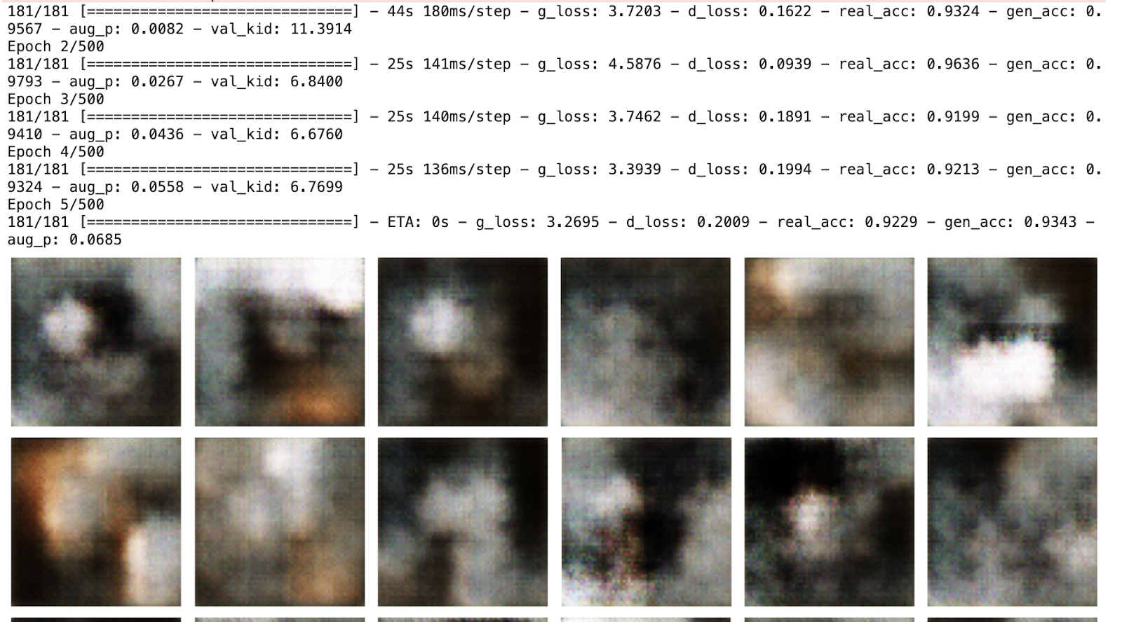
Generated photos

I’ve educated the mannequin for 500 epochs, with the random noise mannequin begins producing these photos on the fifth epoch

After 500 epochs the photographs that is the end result: 

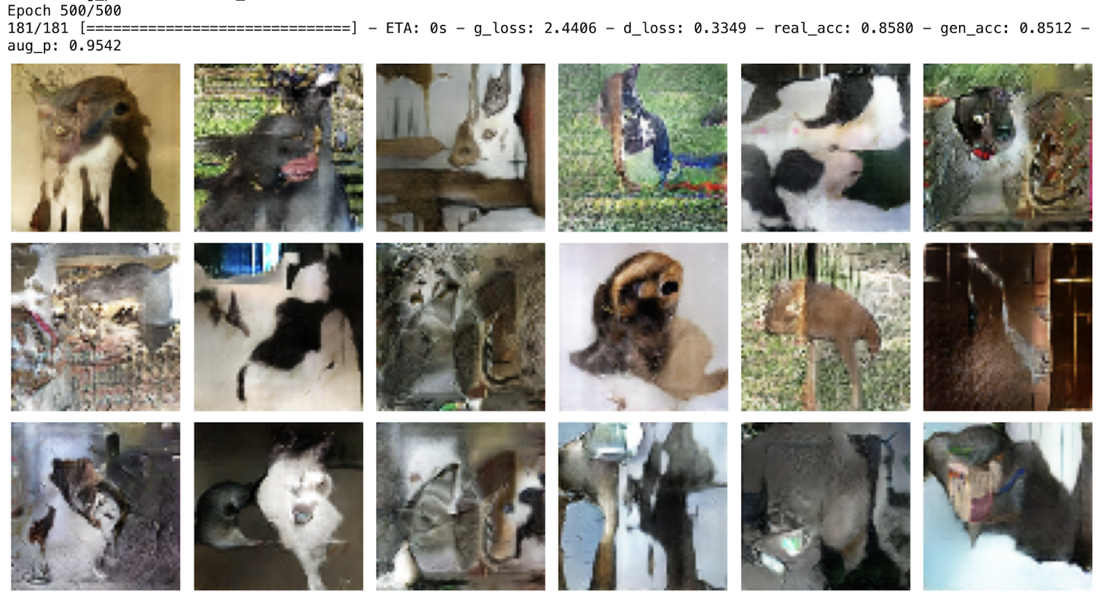
The mannequin must be educated for at the least 6000 epochs earlier than we’d begin seeing clear photos of cats and canines. 

Conclusion

Balancing simplicity and high quality in GAN implementation includes crucial concerns. I like to recommend you select an applicable decision, select the best variety of epochs on your use case, and cautious dealing with of upsampling. You can even use Spectral normalization and dropout layers to reinforce stability and high quality. GANs are tough to take care of, they want a lot of tuning they usually take a variety of time for coaching. Discover newer GANs for higher picture era or you’ll be able to take a look at different probabilistic strategies too. 

Key Takeaways

• Gained insights on the significance of Picture Augmentation.
• Study Mills and Discriminators of GANs and the way to generate new photos.
• Kernel Inception Distance (KID) is a metric used to judge the standard of generated photos primarily based on variations in InceptionV3 community representations.
• GAN structure consists of two important elements: the generator and the discriminator, which work adversarially to generate practical knowledge.
• We Realized and explored to make use of Knowledge Loaders effectively.
• Explored and discovered to work with GANs and practice them.
• TensorFlow gives strong instruments and libraries for implementing GANs for picture era, together with loading datasets, defining fashions, and coaching pipelines.

Often Requested Questions